GKE raises the limit to 512 Pods per node—should you use it?

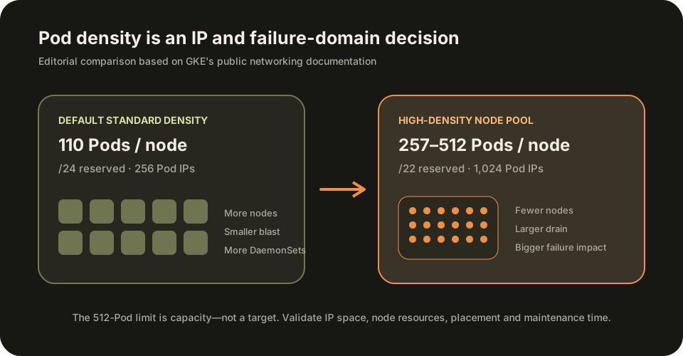
Google Cloud changed a real Kubernetes capacity boundary on 25 September 2026: GKE Standard clusters now support up to 512 Pods per node, double the previous limit of 256. For nodes configured between 257 and 512 Pods, GKE allocates a `/22` Pod CIDR—1,024 IP addresses—to that node.

The headline sounds like an invitation to pack more workloads onto fewer machines. It is better read as an additional design option. Pod density connects node sizing, secondary IP ranges, DaemonSet overhead, scheduling, maintenance duration and the number of workloads lost with one node. The limit tells you what GKE can support; it does not tell you what your service-level objectives should choose.

What changed—and what did not

The new ceiling applies to GKE Standard. The default maximum remains 110 Pods per node, which normally reserves a `/24` range containing 256 Pod addresses for each node. GKE Autopilot still chooses a value dynamically up to 256 and does not let operators configure the setting.

The maximum Pods configuration guide says the value is chosen when a Standard cluster or node pool is created and cannot be changed afterward. Existing pools do not become 512-Pod pools merely because the platform limit increased. Adoption means creating a new node pool with the intended density and moving workloads deliberately.

This is also a scheduling limit, not a promise that CPU, memory, disk, network or kubelet capacity can sustain 512 copies of an arbitrary workload. System Pods consume slots, and each application's requests, limits, sidecars, probes, log volume and connection count determine the practical ceiling.

The IP math becomes the first constraint

GKE uses VPC-native alias IP ranges so every Pod receives a unique address. The per-node range intentionally contains at least twice as many addresses as the configured maximum: 110 Pods use `/24` with 256 addresses; 129–256 use `/23` with 512; and 257–512 use `/22` with 1,024.

That choice changes how many node blocks fit inside the cluster's secondary Pod range. A `/16` contains 65,536 addresses. Dividing it into `/24` blocks yields 256 theoretical node blocks, while `/22` yields only 64. These are address-allocation counts before other GKE quotas and real capacity limits—not a cluster-size guarantee.

A team that enables 512 to reduce node count can therefore exhaust its Pod secondary range sooner if autoscaling still needs many nodes. Inspect the existing secondary range, other node pools and growth headroom first. GKE supports adding discontiguous Pod ranges, but that is a network design decision, not a substitute for sizing the original pool.

Why high density can be attractive

Every Kubernetes node carries fixed overhead: an operating system, kubelet, container runtime, monitoring and security agents, and usually several DaemonSet Pods. Packing lightweight application Pods onto fewer large nodes can reduce that duplicated cost. It can also help workloads with hundreds of tiny, homogeneous workers when nodes have spare resources but the old Pod count ceiling forced the autoscaler to add machines.

The economics depend on the workload. A service-mesh sidecar may use more memory and connections than the application container. Log and security agents may process every container stream. Image pulls, ephemeral storage and DNS lookups can become the binding resources before CPU requests fill the node. Measure the whole per-Pod footprint, not only the main container's request.

Google's networking best practices recommend nodes with at least 16 CPU cores when configuring more than the default 110 Pods. Its large-cluster planning guide gives a further sizing signal of at least one vCPU per ten Pods and notes that the 512 limit assumes an average of no more than two containers per Pod. These are planning guides, not proof that a particular 16-core node is safe at 512.

The operational blast radius grows

If one node hosts 80 Pods, a node loss asks the rest of the cluster to reschedule roughly 80 workloads. At 500, the same failure creates a much larger recovery wave: more pending Pods, image pulls, endpoint updates, DNS traffic, storage attaches and cold starts. Capacity saved during normal operation must be balanced with enough spare capacity to absorb that wave.

Voluntary maintenance also becomes heavier. Kubernetes drain uses the Eviction API and respects PodDisruptionBudgets, so a dense node with many protected workloads can take longer to empty or can block on incompatible budgets. An involuntary node-pressure eviction is different and may not respect the application's PDB. Density therefore makes both the happy maintenance path and the hard failure path important tests.

Replica placement is the second protection. Topology spread constraints can keep replicas distributed across hostnames and zones instead of allowing a high-capacity node to collect most of one service. PDBs limit voluntary concurrent disruption, but they do not spread Pods and do not restore missing capacity. Use both for different jobs.

A safe high-density node-pool rollout

Start with a dedicated canary pool, not a cluster-wide switch. Select stateless, lightweight workloads with multiple replicas, bounded startup time and no fragile local-disk dependency. Keep databases, quorum systems and latency-sensitive agents out of the first migration.

gcloud container node-pools create density-canary \
  --cluster=production \
  --max-pods-per-node=512 \
  --machine-type=<large-machine-type> \
  --num-nodes=<small-canary-count>

Confirm the exact command and supported machine type for the target region and release channel before execution. Label and taint the new pool so only selected workloads enter it. Move one deployment at a time, preserving a rollback path to the old pool.

Observe node CPU and memory, kubelet and runtime resource use, Pod startup latency, DNS latency and errors, connection tracking, CNI behavior, image and ephemeral-storage pressure, log-agent throughput, pending Pods, autoscaler decisions and per-node Pod count. Then run two controlled exercises: drain one dense node under normal budgets, and simulate loss of one node while the cluster has realistic peak traffic.

Success is not “we scheduled 512.” It is that application latency stays within its objective, replacement Pods start inside the recovery target, the remaining pools have headroom, and the network and observability stack remain stable during churn.

Capacity planning checklist

Calculate address space per pool before node resources. At 512 configured Pods, budget a `/22` for every possible node, including surge capacity during upgrades. Verify that cluster autoscaler maximums cannot create more nodes than the Pod range can address.

Next, model the node as a failure domain. Count replicas from the same service that can land together, enforce hostname and zone spread where needed, and ensure a single-node loss does not exceed error-budget assumptions. Check PDBs against actual replica counts and test drain duration rather than assuming the manifests are sufficient.

Finally, include fixed and variable overhead: DaemonSets per node, sidecars per Pod, containers per Pod, image storage, open connections, logs and metrics. A higher limit can reduce fixed per-node cost while increasing variable per-Pod pressure. The optimal point is usually below the hard maximum.

When 512 makes sense

The option fits fleets of small stateless services, event consumers, CI workers or lightweight multi-tenant workloads running on large machines, especially where DaemonSet overhead or the previous 256 limit caused premature node scale-out. It can also help specialized batch pools that tolerate concentrated restarts.

It is a poor default for mixed clusters with uncertain resource requests, large sidecars, stateful workloads, long termination periods or weak topology controls. If Pod IP conservation is the goal, higher density actually reserves more addresses per node; lowering the maximum Pods per node preserves address space for more nodes.

The practical decision is to treat 512 as a new upper bound for a specifically engineered pool. Create a fresh pool, prove its IP plan, size large nodes from measured per-Pod overhead, spread replicas, test drain and loss, and retain rollback capacity. GKE expanded the design space; reliable platform engineering still chooses the operating point.

Prepared by: Noor Yasser